Tutorial - Phylo2Vec Workshop

Welcome to the Phylo2Vec demo! Here, we will quickly visit the main functions of phylo2vec, including:

A primer on computational phylogenetics, running popular software such as rapidNJ and IQ-TREE for inferring trees from molecular sequences
Visualising trees using ete3 or Biopython
Using basic phylo2vec functions: sam trees, converting trees to the phylo2vec format, performing operations on trees
Using modern tools and infrastructure present in the phylo2vec package: pixi, pytest, and pytest-benchmark

# Constants

data_dir = "../data"
tree_dir = "../trees"

What is phylo2vec?¶

phylo2vec is a library for encoding and manipulating binary (phylogenetic) trees under a compact vector format. In its current version, the library is useful for:

Sampling random trees
Fast comparison of trees
Compressing trees or files with many trees

The current version of Phylo2Vec (1.x) relies on a core written in Rust, with bindings to Python and R. That means that you do not need to know Rust to use the package, Python or R are sufficient! To become more familiar with Rust, we recommend this interactive book.

Before we get started, we will quickly introduce pixi, the package manger we use to orchestrate dependencies in this workshop (and in the phylo2vec package).

A minimal pixi cheatsheet¶

Pixi is a past package manager built on top of the conda ecosystem. By default, it resolves packages from conda-forge, a community-driven channel with the most complete, up-to-date collection of scientific and data packages.

For the workshop (19.09.2025), installations are done for you via GitHub codespaces! However, if you want to run this notebook independently, you may either:

Install the dependencies separately (not recommended)
Use pixi to manage everything in a reproducible and isolated way

We will here briefly go through pixi basics: installing it, creating a pixi.toml, managing dependencies, and running scripts

Installing pixi¶

curl -fsSL https://pixi.sh/install.sh | bash

Creating a new project¶

pixi init

Adding dependencies¶

pixi add numpy pandas matplotlib
pixi remove matplotlib
pixi add bioconda::rapidnj # Channel specification for conda packages
pixi add r-ggplot2 # Adding an R package

Setting up a pixi.toml for a project¶

Here is a minimal file to create a custom project

[project]
name = "pixi-workshop"
version = "0.1.0"
description = "Minimal pixi project for the 19.09.2025 workshop"
channels = ["conda-forge", "bioconda", "r"]

[dependencies]
python = ">=3.11,<3.13"
numpy = "*"
pandas = "*"
bioconda::rapidnj = "*"
r-ggplot2 = "*"

Running scripts¶

Define scripts in your pixi.toml, e.g.:

[scripts]
start = "python main.py"
notebook = "jupyter lab"

and run them with:

pixi run start
pixi run notebook

You may also run executables via pixi run, e.g., pixi run rapidnj

Activating an environment¶

If you want a shell with all dependencies available:

pixi shell

A short primer on phylogenetics¶

The overarching goal of phylogenetics is to study the evolutionary history between different entities (e.g., animal species, viral strains, languages...) using observable data.

The main artefact of phylogenetics is a phylogenetic tree, a diagram which describe the evolutionary relationships between the entities of interest. A phylogenetic tree shares many similarities with the notion of trees defined in graph theory/computer science:

It connects vertices (or nodes) with edges (or branches).
It is acyclic
Any two nodes in a tree are connected by a unique path.
Terminal nodes, or leaves correspond to observable species (with observable data)
Internal nodes, or ancestral nodes correspond to unobserved species. They are inferred using inference algorithms
Edges, or branches connect nodes and may have variable lengths (branch lengths). In phylogenetics, branch lengths may represent time, or the amount of evolution between a parent node and its child.

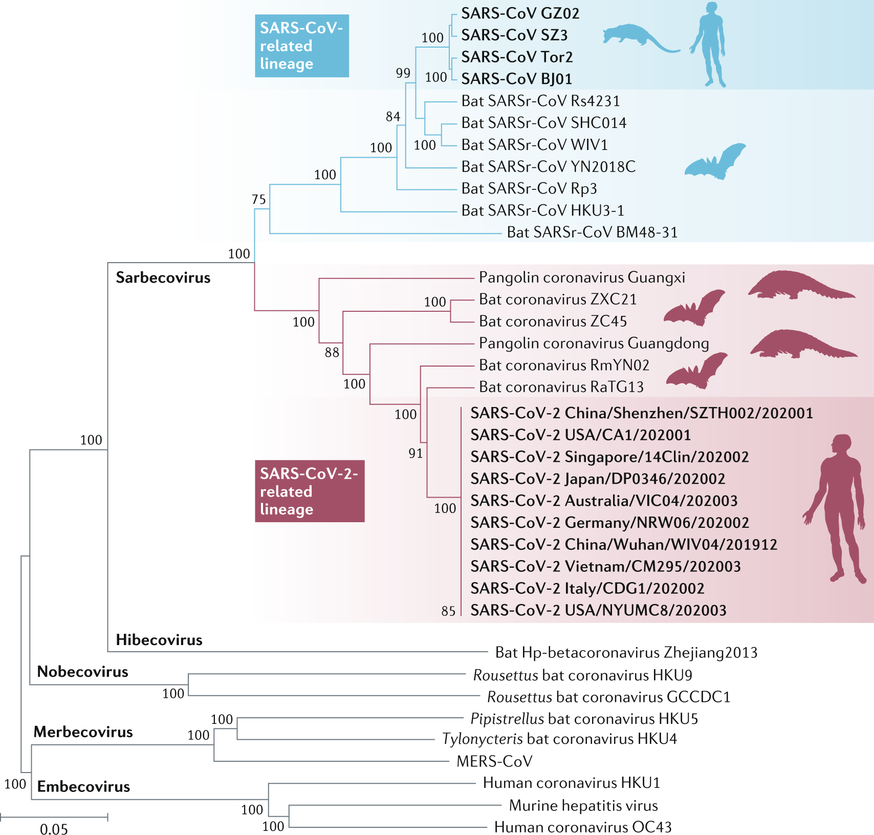
In the tree below, different species of coronaviruses are mapped, highlighting the different genera (Sarbecovirus, Hibecovirus, Embecovirus, etc.). Tree tips correspond to different viral strains, and internal nodes correspond to unobserved ancestors, inferred from the data at hand.

Source: https://www.nature.com/articles/s41579-020-00459-7

Most modern phylogenetic analyses rely on molecular data, as it provides a precise and objective measure of evolutionary relationships. Thus phylogeneticists compare DNA, RNA, or protein sequences across entities (or taxa, in biology) to infer common ancestry and divergence times.

A simple genetic analysis requires at least three steps:

Collecting sequences
Aligning sequences
Inferring a phylogenetic tree

Sequence alignment is necessary to compare homologous positions in sequences as genes, and genomes more generally, vary in length.

Within a gene, some entities might present length-altering mutations such as insertions or deletions, or other structural changes.
Across genomes, different organisms may not have the same set of genes, making alignment essential for comparing homologous regions.

For the purpose of this tutorial, we will start with pre-aligned sequences. If interested, see chapter 3 of the book https://decodinggenomes.org, available for free online. Tools include MAFFT, Clustal Omega, FAMSA.

Phylogenetic inference is the task of inferring plausible phylogenetic trees from a molecular sequence alignment (MSA). Several approaches exist:

The simplest is to use distance-based methods, such as neighbor-joining.
- Example tool: rapidNJ
A state-of-the-art method is maximum likelihood, which evaluates how well different trees explain the observed data under a chosen model of sequence evolution.
- Example tools: IQ-TREE, RAxML-NG
Bayesian inference goes further by estimating the probability distribution of trees, incorporating prior information and quantifying uncertainty.
- Example tool: BEAST.

Processing genetic sequences in Python¶

A useful library for manipulating genetic sequence sets in Python is Biopython. We will quickly visualise the first dataset of the workshop, which comprises mitochondrial DNA from (mostly) primates. The sequence is in the FASTA format, whose basic structure looks like this:

>species1
atcgatcgatcg
>species2
tacgtacgtacg
>spescies3
atgcatggatgg

(nucleotides or amino acids may also be uppercase)

from Bio import AlignIO, SeqIO
from collections import Counter

import pandas as pd


def summary(file, format="fasta"):
    aln = AlignIO.read(file, format)

    n_seq = len(aln)
    aln_length = aln.get_alignment_length()

    # Count gaps per column
    gap_fractions = []
    all_counts = []
    conserved_cols = 0
    for i in range(aln_length):
        col = aln[:, i]
        counts = Counter(col)
        _, count = counts.most_common(1)[0]
        if count == n_seq:  # fully conserved
            conserved_cols += 1
        gap_fractions.append(counts.get("-", 0))
        all_counts.append(counts)

    nucleotide_counts = pd.DataFrame(all_counts).fillna(0).astype(int).sum(0).to_dict()

    return {
        "n_sequences": n_seq,
        "alignment_length": aln_length,
        "percent_conserved_sites": conserved_cols / aln_length * 100,
        "percent_gap": sum(gap_fractions) / (n_seq * aln_length) * 100,
        "nucleotide_counts": nucleotide_counts,
    }


summary("../data/primates.fa")

{'n_sequences': 14,
 'alignment_length': 232,
 'percent_conserved_sites': 5.172413793103448,
 'percent_gap': 0.03078817733990148,
 'nucleotide_counts': {'a': 1217, 'c': 1304, 't': 599, 'g': 127, '-': 1}}

Neighbor-joining with rapidNJ¶

Under the neighbour joining framework, we build a tree by iteratively joining pairs of taxa with the smallest evolutionary distance.

rapidNJ is an example tool for very fast neighbour joining. Using pixi we run pixi run rapidnj to run the tool:

!pixi run rapidnj -h

Rapid neighbour-joining. An implementation of the canonical neighbour-joining method which utilize a fast search heuristic to reduce the running time. RapidNJ can be used to reconstruct large trees using a very small amount of memory by utilizing the HDD as storage.

USAGE: rapidnj INPUT [OPTIONS]
The INPUT can be a distance matrix in phylip (.phylip) format or a multiple alignment in stockholm (.sth) or phylip format (.phylip).
OPTIONS:
  -h, --help                display this help message and exit.
  -v, --verbose             turn on verbose output.
  -i, --input-format ARG    Specifies the type of input. pd = distance
                            matrix in phylip format, sth = multiple alignment in (single line) stockholm format.
                            fa = multiple alignment in (single line) FASTA format.
  -o, --output-format ARG   Specifies the type of output. t = phylogenetic tree in newick format
                            (default), m = distance matrix.
  -a, --evolution-model ARG Specifies which sequence evolution method to use when computing
                            distance estimates from multiple alignments. jc = juke cantor,
                            kim = Kimura's distance (default).
  -m, --memory-size         The maximum amount of memory which rapidNJ is allowed to use (in MB).
                            Default is 90% of all available memory.
  -k, --rapidnj-mem ARG     Force RapidNJ to use a memory efficient version of rapidNJ. The 'arg'
                            specifies the percentage of a sorted distance matrix which should be
                            stored in memory (arg=10 means 10%).
  -d, --rapidnj-disk ARG    Force RapidNJ to use HDD caching where 'arg' is the directory used to
                            store cached files.
  -c, --cores ARG           Number of cores to use for computating distance matrices from multiple
                            alignments. All available cores are used by default.
  -b  --bootstrap ARG       Compute bootstrap values using ARG samples. The output tree will be
                            annotated with the bootstrap values.
  -t, --alignment-type ARG  Force the input alignment to be treated as: p = protein alignment, 
                            d = DNA alignment.
  -n  --no-negative-length  Adjust for negative branch lengths.
  -x  --output-file ARG     Output the result to this file instead of stdout.

To get a tree (the default option), we can run:

primate_rapidnj_file = f"{tree_dir}/primates.rapidnj"
!pixi run rapidnj -v $data_dir/primates.fa -x $primate_rapidnj_file

RapidNJ v. 2.2.2ating environment                                                        
64 bit system detected.
Using 128 core(s) for distance estimation
Input format determined as FASTA
Reading data...
Input type determined as DNA.
Number of sequences: 14
Sequence length: 232
Matrix size: 14
257537 MB of memory is available
Using RapidNJ 
Using 0.000747681 MB for distance matrix
Using 0.00149536 MB for sortedMatrix
Total memory consumption is 0.00224304 MB
Computing distance matrix... 
Fastdist is enabled
Using Kimura algorithm to calculate distances
Computing phylogetic tree... 
100.00%

We get here an output in the so-called Newick format.

This format represents taxa using nested parentheses, for example: ((Taxon1:BranchLength1, Taxon2:BranchLength2):BranchLength3);. Subtrees are enclosed recursively in parentheses, and every tree ends with a semicolon (;).

!cat $tree_dir/primates.rapidnj

(('Tarsier':0.42099,'Lemur':0.36721):0.101,((((((('Human':0.11568,'Chimp':0.17827):0.088192,'Gorilla':0.11228):0.066043,'Orang':0.20108):0.068184,'Gibbon':0.30113):0.045591,((('RhesusMac':0.066186,'JpnMacaq':0.038473):0.032833,'CrabEMac':0.17245):0.11606,'BarbMacaq':0.1742):0.14558):0.08527,'SquirMonk':0.38666):0.06142,'Mouse':0.5341):0.017041,'Bovine':0.34356);

Although not immediately easy to read, we can observe that:

✅ Great apes (Humans, Chimpanzees, Gorillas, Orangutans) form a separate clade, as expected.
Macaques branch off later (Rhesus Macaque, Japanese Macaque, Crab-eating Macaque).
❌ Bovine appears as the most basal lineage relative to this primate set, which does not reflect the accepted mammalian phylogeny
❌ The placement of the Squirrel Monkey deep within the tree is also unusual.

Maximum likelihood with IQ-TREE¶

Under the maximum likelihood framework, we build a tree by finding the topology and branch lengths that maximize the probability of observing the given sequence alignment under a specified model of sequence evolution. The optimal tree is identified by exploring possible tree topologies using many tree rearrangements and selecting the one with the highest likelihood score.

IQ-TREE is an example tool for fast maximum likelihood estimation. For a detailed tutorial on IQ-TREE see this tutorial. Using pixi we run pixi run iqtree to run the tool:

!pixi run iqtree -h | head -n 50

IQ-TREE version 3.0.1 for Linux x86 64-bit built Jul  9 2025                             
Developed by Bui Quang Minh, Thomas Wong, Nhan Ly-Trong, Huaiyan Ren
Contributed by Lam-Tung Nguyen, Dominik Schrempf, Chris Bielow,
Olga Chernomor, Michael Woodhams, Diep Thi Hoang, Heiko Schmidt

Usage: iqtree [-s ALIGNMENT] [-p PARTITION] [-m MODEL] [-t TREE] ...

GENERAL OPTIONS:
  -h, --help           Print (more) help usages
  -s FILE[,...,FILE]   PHYLIP/FASTA/NEXUS/CLUSTAL/MSF alignment file(s)
  -s DIR               Directory of alignment files
  --seqtype STRING     BIN, DNA, AA, NT2AA, CODON, MORPH (default: auto-detect)
  -t FILE|PARS|RAND    Starting tree (default: 99 parsimony and BIONJ)
  -o TAX[,...,TAX]     Outgroup taxon (list) for writing .treefile
  --prefix STRING      Prefix for all output files (default: aln/partition)
  --seed NUM           Random seed number, normally used for debugging purpose
  --safe               Safe likelihood kernel to avoid numerical underflow
  --mem NUM[G|M|%]     Maximal RAM usage in GB | MB | %
  --runs NUM           Number of indepedent runs (default: 1)
  -v, --verbose        Verbose mode, printing more messages to screen
  -V, --version        Display version number
  --quiet              Quiet mode, suppress printing to screen (stdout)
  -fconst f1,...,fN    Add constant patterns into alignment (N=no. states)
  --epsilon NUM        Likelihood epsilon for parameter estimate (default 0.01)
  -T NUM|AUTO          No. cores/threads or AUTO-detect (default: 1)
  --threads-max NUM    Max number of threads for -T AUTO (default: all cores)

CHECKPOINT:
  --redo               Redo both ModelFinder and tree search
  --redo-tree          Restore ModelFinder and only redo tree search
  --undo               Revoke finished run, used when changing some options
  --cptime NUM         Minimum checkpoint interval (default: 60 sec and adapt)

PARTITION MODEL:
  -p FILE|DIR          NEXUS/RAxML partition file or directory with alignments
                       Edge-linked proportional partition model
  -q FILE|DIR          Like -p but edge-linked equal partition model 
  -Q FILE|DIR          Like -p but edge-unlinked partition model
  -S FILE|DIR          Like -p but separate tree inference
  --subsample NUM      Randomly sub-sample partitions (negative for complement)
  --subsample-seed NUM Random number seed for --subsample

LIKELIHOOD/QUARTET MAPPING:
  --lmap NUM           Number of quartets for likelihood mapping analysis
  --lmclust FILE       NEXUS file containing clusters for likelihood mapping
  --quartetlh          Print quartet log-likelihoods to .quartetlh file

TREE SEARCH ALGORITHM:
  --ninit NUM          Number of initial parsimony trees (default: 100)
  --ntop NUM           Number of top initial trees (default: 20)

primate_iqtree_prefix = f"{tree_dir}/primates"
!pixi run iqtree -s $data_dir/primates.fa -m GTR+G --prefix $primate_iqtree_prefix --redo
primate_iqtree_file = f"{primate_iqtree_prefix}.treefile"

IQ-TREE version 3.0.1 for Linux x86 64-bit built Jul  9 2025                             
Developed by Bui Quang Minh, Thomas Wong, Nhan Ly-Trong, Huaiyan Ren
Contributed by Lam-Tung Nguyen, Dominik Schrempf, Chris Bielow,
Olga Chernomor, Michael Woodhams, Diep Thi Hoang, Heiko Schmidt

Host:    didelx02 (AVX2, FMA3, 251 GB RAM)
Command: /home/nclow23/src/phylo2vec/workshop/.pixi/envs/default/bin/iqtree -s ../data/primates.fa -m GTR+G --prefix ../trees/primates --redo
Seed:    693600 (Using SPRNG - Scalable Parallel Random Number Generator)
Time:    Thu Sep 18 16:42:20 2025
Kernel:  AVX+FMA - 1 threads (128 CPU cores detected)

HINT: Use -nt option to specify number of threads because your CPU has 128 cores!
HINT: -nt AUTO will automatically determine the best number of threads to use.

Reading alignment file ../data/primates.fa ... Fasta format detected
Reading fasta file: done in 7.88001e-05 secs
Alignment most likely contains DNA/RNA sequences
Constructing alignment: done in 0.000204699 secs
Alignment has 14 sequences with 232 columns, 217 distinct patterns
191 parsimony-informative, 29 singleton sites, 12 constant sites
           Gap/Ambiguity  Composition  p-value
Analyzing sequences: done in 9.19681e-06 secs
   1  Mouse        0.00%    failed      3.42%
   2  Bovine       0.00%    passed     10.27%
   3  Lemur        0.00%    passed     17.69%
   4  Tarsier      0.00%    failed      3.53%
   5  SquirMonk    0.43%    passed      8.42%
   6  JpnMacaq     0.00%    passed     85.47%
   7  RhesusMac    0.00%    passed     96.42%
   8  CrabEMac     0.00%    passed     46.18%
   9  BarbMacaq    0.00%    passed     75.38%
  10  Gibbon       0.00%    passed      6.16%
  11  Orang        0.00%    failed      0.83%
  12  Gorilla      0.00%    passed     20.22%
  13  Chimp        0.00%    passed     38.37%
  14  Human        0.00%    passed     17.55%
****  TOTAL        0.03%  3 sequences failed composition chi2 test (p-value<5%; df=3)
Checking for duplicate sequences: done in 2.98675e-05 secs

Create initial parsimony tree by phylogenetic likelihood library (PLL)... 0.000 seconds

NOTE: 0 MB RAM (0 GB) is required!
Estimate model parameters (epsilon = 0.100)
1. Initial log-likelihood: -3001.337
2. Current log-likelihood: -2659.176
3. Current log-likelihood: -2632.929
4. Current log-likelihood: -2626.155
5. Current log-likelihood: -2623.111
6. Current log-likelihood: -2621.219
7. Current log-likelihood: -2619.644
8. Current log-likelihood: -2618.263
9. Current log-likelihood: -2617.070
10. Current log-likelihood: -2616.045
11. Current log-likelihood: -2615.173
12. Current log-likelihood: -2614.445
13. Current log-likelihood: -2613.812
14. Current log-likelihood: -2613.296
15. Current log-likelihood: -2612.851
16. Current log-likelihood: -2612.498
17. Current log-likelihood: -2612.180
18. Current log-likelihood: -2611.917
19. Current log-likelihood: -2611.687
20. Current log-likelihood: -2611.505
21. Current log-likelihood: -2611.354
22. Current log-likelihood: -2611.228
23. Current log-likelihood: -2611.114
Optimal log-likelihood: -2610.990
Rate parameters:  A-C: 0.12392  A-G: 8.40821  A-T: 0.04733  C-G: 0.00010  C-T: 3.90865  G-T: 1.00000
Warning! Some parameters hit the boundaries
Base frequencies:  A: 0.375  C: 0.402  G: 0.039  T: 0.184
Gamma shape alpha: 2.813
Parameters optimization took 23 rounds (0.100 sec)
Wrote distance file to... 
Computing ML distances based on estimated model parameters...
Calculating distance matrix: done in 0.00100836 secs using 99.96% CPU
Computing ML distances took 0.001051 sec (of wall-clock time) 0.001054 sec (of CPU time)
WARNING: Some pairwise ML distances are too long (saturated)
Setting up auxiliary I and S matrices: done in 6.37015e-05 secs using 98.9% CPU
Constructing RapidNJ tree: done in 8.59043e-05 secs using 98.95% CPU
Computing RapidNJ tree took 0.000918 sec (of wall-clock time) 0.000915 sec (of CPU time)
Log-likelihood of RapidNJ tree: -2610.865
--------------------------------------------------------------------
|             INITIALIZING CANDIDATE TREE SET                      |
--------------------------------------------------------------------
Generating 98 parsimony trees... 0.034 second
Computing log-likelihood of 98 initial trees ... 0.066 seconds
Current best score: -2610.865

Do NNI search on 20 best initial trees
Optimizing NNI: done in 0.00500681 secs using 98.33% CPU
Estimate model parameters (epsilon = 0.100)
BETTER TREE FOUND at iteration 1: -2610.032
Optimizing NNI: done in 0.00497145 secs using 99.97% CPU
Optimizing NNI: done in 0.00909396 secs using 90.03% CPU
Optimizing NNI: done in 0.00685458 secs using 58.41% CPU
Optimizing NNI: done in 0.0071691 secs using 99.98% CPU
Optimizing NNI: done in 0.00957553 secs using 99.99% CPU
Optimizing NNI: done in 0.00696315 secs using 99.87% CPU
Optimizing NNI: done in 0.00915112 secs using 99.99% CPU
Optimizing NNI: done in 0.011732 secs using 99.83% CPU
UPDATE BEST LOG-LIKELIHOOD: -2610.030
Optimizing NNI: done in 0.00593418 secs using 99.98% CPU
Iteration 10 / LogL: -2610.154 / Time: 0h:0m:0s
Optimizing NNI: done in 0.0109777 secs using 99.98% CPU
Optimizing NNI: done in 0.00736925 secs using 99.98% CPU
Optimizing NNI: done in 0.00739731 secs using 99.98% CPU
Optimizing NNI: done in 0.0104288 secs using 53.16% CPU
UPDATE BEST LOG-LIKELIHOOD: -2610.030
Optimizing NNI: done in 0.0122123 secs using 76.82% CPU
Optimizing NNI: done in 0.00585278 secs using 99.85% CPU
Optimizing NNI: done in 0.00853844 secs using 99.94% CPU
Optimizing NNI: done in 0.00760107 secs using 99.99% CPU
Optimizing NNI: done in 0.0119562 secs using 99.99% CPU
UPDATE BEST LOG-LIKELIHOOD: -2610.030
Optimizing NNI: done in 0.00815403 secs using 99.98% CPU
Iteration 20 / LogL: -2610.436 / Time: 0h:0m:0s
Finish initializing candidate tree set (3)
Current best tree score: -2610.030 / CPU time: 0.276
Number of iterations: 20
--------------------------------------------------------------------
|               OPTIMIZING CANDIDATE TREE SET                      |
--------------------------------------------------------------------
Optimizing NNI: done in 0.00671408 secs using 99.98% CPU
Optimizing NNI: done in 0.00298279 secs using 99.97% CPU
Optimizing NNI: done in 0.00676535 secs using 99.98% CPU
Optimizing NNI: done in 0.0111015 secs using 99.98% CPU
Optimizing NNI: done in 0.00400995 secs using 99.95% CPU
Optimizing NNI: done in 0.00785762 secs using 99.83% CPU
Optimizing NNI: done in 0.00635632 secs using 99.98% CPU
Optimizing NNI: done in 0.0104368 secs using 99.99% CPU
Optimizing NNI: done in 0.0114346 secs using 99.99% CPU
Optimizing NNI: done in 0.00570496 secs using 99.98% CPU
Iteration 30 / LogL: -2610.053 / Time: 0h:0m:0s (0h:0m:1s left)
Optimizing NNI: done in 0.0093823 secs using 78.07% CPU
Optimizing NNI: done in 0.00635486 secs using 74.24% CPU
Optimizing NNI: done in 0.00536266 secs using 99.84% CPU
Optimizing NNI: done in 0.00743499 secs using 99.49% CPU
Optimizing NNI: done in 0.00751443 secs using 99.98% CPU
Optimizing NNI: done in 0.00419564 secs using 99.98% CPU
Optimizing NNI: done in 0.0148444 secs using 99.95% CPU
Optimizing NNI: done in 0.00868989 secs using 99.99% CPU
Optimizing NNI: done in 0.00615883 secs using 85.36% CPU
Optimizing NNI: done in 0.0124211 secs using 44.92% CPU
Iteration 40 / LogL: -2618.101 / Time: 0h:0m:0s (0h:0m:0s left)
Optimizing NNI: done in 0.00765366 secs using 99.85% CPU
Optimizing NNI: done in 0.0101386 secs using 99.99% CPU
Optimizing NNI: done in 0.0064139 secs using 99.99% CPU
Optimizing NNI: done in 0.0103929 secs using 99.98% CPU
Optimizing NNI: done in 0.00854854 secs using 99.98% CPU
Optimizing NNI: done in 0.00640678 secs using 99.99% CPU
Optimizing NNI: done in 0.00802007 secs using 99.99% CPU
Optimizing NNI: done in 0.0068227 secs using 99.98% CPU
Optimizing NNI: done in 0.010516 secs using 99.99% CPU
Optimizing NNI: done in 0.00393656 secs using 99.96% CPU
Iteration 50 / LogL: -2610.425 / Time: 0h:0m:0s (0h:0m:0s left)
Optimizing NNI: done in 0.0123437 secs using 99.99% CPU
Optimizing NNI: done in 0.00637322 secs using 99.98% CPU
Optimizing NNI: done in 0.00842124 secs using 99.99% CPU
Optimizing NNI: done in 0.00787973 secs using 99.98% CPU
Optimizing NNI: done in 0.00774104 secs using 64.98% CPU
Optimizing NNI: done in 0.0100273 secs using 90.4% CPU
Optimizing NNI: done in 0.00957386 secs using 99.98% CPU
Optimizing NNI: done in 0.00665596 secs using 99.97% CPU
Optimizing NNI: done in 0.00632735 secs using 99.98% CPU
Optimizing NNI: done in 0.0124287 secs using 99.95% CPU
Iteration 60 / LogL: -2610.065 / Time: 0h:0m:0s (0h:0m:0s left)
Optimizing NNI: done in 0.00458817 secs using 99.97% CPU
Optimizing NNI: done in 0.00596374 secs using 99.97% CPU
Optimizing NNI: done in 0.00791236 secs using 99.98% CPU
Optimizing NNI: done in 0.00618777 secs using 99.97% CPU
Optimizing NNI: done in 0.00751405 secs using 99.97% CPU
Optimizing NNI: done in 0.00435716 secs using 99.97% CPU
Optimizing NNI: done in 0.00629161 secs using 38.38% CPU
Optimizing NNI: done in 0.00544595 secs using 98.62% CPU
Optimizing NNI: done in 0.00666339 secs using 99.98% CPU
Optimizing NNI: done in 0.00981522 secs using 99.99% CPU
Iteration 70 / LogL: -2610.160 / Time: 0h:0m:0s (0h:0m:0s left)
Optimizing NNI: done in 0.0121924 secs using 99.89% CPU
Optimizing NNI: done in 0.00755304 secs using 99.99% CPU
Optimizing NNI: done in 0.00906553 secs using 99.98% CPU
Optimizing NNI: done in 0.00748861 secs using 99.98% CPU
Optimizing NNI: done in 0.00550761 secs using 99.97% CPU
Optimizing NNI: done in 0.012251 secs using 99.98% CPU
Optimizing NNI: done in 0.00825837 secs using 99.97% CPU
Optimizing NNI: done in 0.00588506 secs using 99.97% CPU
Optimizing NNI: done in 0.0115544 secs using 99.98% CPU
Optimizing NNI: done in 0.00828556 secs using 99.98% CPU
Iteration 80 / LogL: -2610.380 / Time: 0h:0m:0s (0h:0m:0s left)
Optimizing NNI: done in 0.00682278 secs using 99.97% CPU
Optimizing NNI: done in 0.00439005 secs using 99.95% CPU
UPDATE BEST LOG-LIKELIHOOD: -2610.030
Optimizing NNI: done in 0.00862168 secs using 99.98% CPU
Optimizing NNI: done in 0.0126455 secs using 99.98% CPU
Optimizing NNI: done in 0.00639279 secs using 99.97% CPU
Optimizing NNI: done in 0.0101662 secs using 99.99% CPU
Optimizing NNI: done in 0.00707069 secs using 99.99% CPU
Optimizing NNI: done in 0.0078156 secs using 99.97% CPU
Optimizing NNI: done in 0.00773664 secs using 99.98% CPU
Optimizing NNI: done in 0.00642268 secs using 99.97% CPU
Iteration 90 / LogL: -2610.063 / Time: 0h:0m:0s (0h:0m:0s left)
Optimizing NNI: done in 0.0133875 secs using 99.99% CPU
Optimizing NNI: done in 0.00618097 secs using 99.98% CPU
Optimizing NNI: done in 0.0087916 secs using 99.97% CPU
Optimizing NNI: done in 0.0051278 secs using 99.98% CPU
Optimizing NNI: done in 0.00642028 secs using 99.98% CPU
Optimizing NNI: done in 0.0101127 secs using 22.48% CPU
Optimizing NNI: done in 0.0132855 secs using 98.96% CPU
Optimizing NNI: done in 0.00985405 secs using 99.98% CPU
Optimizing NNI: done in 0.00607071 secs using 99.97% CPU
Optimizing NNI: done in 0.00968047 secs using 99.97% CPU
Iteration 100 / LogL: -2610.523 / Time: 0h:0m:1s (0h:0m:0s left)
Optimizing NNI: done in 0.0111642 secs using 99.99% CPU
Optimizing NNI: done in 0.00608087 secs using 99.97% CPU
TREE SEARCH COMPLETED AFTER 102 ITERATIONS / Time: 0h:0m:1s

--------------------------------------------------------------------
|                    FINALIZING TREE SEARCH                        |
--------------------------------------------------------------------
Performs final model parameters optimization
Estimate model parameters (epsilon = 0.010)
1. Initial log-likelihood: -2610.030
2. Current log-likelihood: -2609.993
3. Current log-likelihood: -2609.942
4. Current log-likelihood: -2609.895
5. Current log-likelihood: -2609.857
6. Current log-likelihood: -2609.826
7. Current log-likelihood: -2609.800
8. Current log-likelihood: -2609.779
9. Current log-likelihood: -2609.761
Optimal log-likelihood: -2609.751
Rate parameters:  A-C: 0.10467  A-G: 8.42079  A-T: 0.03803  C-G: 0.00010  C-T: 3.89572  G-T: 1.00000
Warning! Some parameters hit the boundaries
Base frequencies:  A: 0.375  C: 0.402  G: 0.039  T: 0.184
Gamma shape alpha: 2.716
Parameters optimization took 9 rounds (0.035 sec)
BEST SCORE FOUND : -2609.751
Total tree length: 35.893

Total number of iterations: 102
CPU time used for tree search: 0.916 sec (0h:0m:0s)
Wall-clock time used for tree search: 0.958 sec (0h:0m:0s)
Total CPU time used: 1.070 sec (0h:0m:1s)
Total wall-clock time used: 1.110 sec (0h:0m:1s)

Analysis results written to: 
  IQ-TREE report:                ../trees/primates.iqtree
  Maximum-likelihood tree:       ../trees/primates.treefile
  Likelihood distances:          ../trees/primates.mldist
  Screen log file:               ../trees/primates.log

Date and Time: Thu Sep 18 16:42:21 2025

!cat $tree_dir/primates.treefile

(Mouse:8.3557270836,((Bovine:2.5963494542,Lemur:4.8260218164):1.1363701356,Tarsier:5.3614256276):0.8929574644,(SquirMonk:2.9417796358,((JpnMacaq:0.0000029242,(RhesusMac:0.0964657866,(CrabEMac:0.1339703904,BarbMacaq:0.5369865414):0.1170784582):0.0205794511):1.4487558401,(Gibbon:1.3183092356,(Orang:0.8632011204,(Gorilla:0.1681777496,(Chimp:0.2545481157,Human:0.1205079715):0.2193569261):0.2118140431):0.4130042967):1.0934384331):0.9379140845):1.8281193536);

This tree seems already more plausible:

✅ Mouse is the outgroup, far outside the other mammals, which makes sense given its divergence.
✅ Squirrel Monkey separates next, rather than clustering with other New World monkeys
✅ Old World monkeys (Japanese Macaque, Rhesus Macaque, Crab-eating Macaque, Barbary Macaque) form a nested clade
✅ Apes (Gibbon, Orangutan, Gorilla, Chimpanzee, Human) form a well-supported, nested clade
Bovine and Lemur form a clade that branches off early: unusual (bovines are not primates)
Tarsier is slightly more derived than the Bovine–Lemur clade, which is also somewhat unexpected.

Factors that could enhance the accuracy of the tree include the choice of evolutionary model and, most importantly, the quality of the data. Here, our dataset is minuscule (232 base pairs!), so more data, for example by including more genes, would greatly improve our ability to reconstruct a plausible evolutionary history.

Visualizing trees¶

Several libraries in python already exist to visualize trees. A popular library is ete.

To have an ASCII drawing of the tree (without branch lengths represented), simply use print

# import PyQt5
from ete3 import Tree

# Load a tree from a Newick file*
primate_iqtree_tree = Tree(primate_iqtree_file)

# Print the tree in ASCII format
print(primate_iqtree_tree)


   /-Mouse
  |
  |      /-Bovine
  |   /-|
  |--|   \-Lemur
--|  |
  |   \-Tarsier
  |
  |   /-SquirMonk
  |  |
  |  |      /-JpnMacaq
   \-|   /-|
     |  |  |   /-RhesusMac
     |  |   \-|
     |  |     |   /-CrabEMac
      \-|      \-|
        |         \-BarbMacaq
        |
        |   /-Gibbon
         \-|
           |   /-Orang
            \-|
              |   /-Gorilla
               \-|
                 |   /-Chimp
                  \-|
                     \-Human

Interactive visualisations are also possible using primate_iqtree_tree.show(). They require PyQt5 (pixi add --pypi PyQt5) and may crash your notebook.

We provide here a small function to plot a tree from an ete3 Tree in matplotlib.

import itertools

import matplotlib.pyplot as plt
import numpy as np
from matplotlib.collections import LineCollection


def plot_tree(
    tree,
    align_names=False,
    name_offset=None,
    fontsize=9,
    cdict=None,
    outgroup=None,
    ax=None,
):
    """
    Plots a ete3.Tree object using matploltib.

    Adapted from: https://gist.github.com/jolespin/5d90deff552138d73de7ed4bdd9ac57a

    Parameters
    ----------
    tree : str
        An ete3.Tree object
    align_names: bool
        If True names will be aligned vertically, by default False
    name_offset : float, optional
        Offset relative to tips to write leaf_names. In BL scale, by default None
    fontsize : int, optional
        Text font size, by default 9
    ax : matplotlib.Axes object, optional
        Object on which the tree will be plotted, by default None

    Returns
    -------
    ax : matplotlib.Axes object
        The matplotlib axis containing the drawn tree
    """
    if outgroup is not None:
        if isinstance(outgroup, list):
            outgroup = tree.get_common_ancestor(outgroup)
        tree.set_outgroup(outgroup)

    if ax is None:
        ax = plt.gca()

    aligned_lines = []

    max_x = max(n.get_distance(tree) for n in tree.iter_leaves())

    if name_offset is None:
        name_offset = max_x / 50.0

    node_pos = {n2: i for i, n2 in enumerate(tree.get_leaves()[::-1])}
    node_list = itertools.chain(tree.iter_descendants(strategy="postorder"), [tree])

    # draw tree
    for node in node_list:
        # Parent style
        # pstyle = node.img_style

        x = sum(n2.dist for n2 in node.iter_ancestors()) + node.dist

        if node.is_leaf():
            y = node_pos[node]
            if align_names:
                x = max_x
                aligned_lines.append(((x, y), (max_x + name_offset, y)))

        else:
            y = np.mean([node_pos[n2] for n2 in node.children])
            node_pos[node] = y

            # draw vertical line
            ax.plot(
                [x, x],
                [node_pos[node.children[0]], node_pos[node.children[-1]]],
                c="k",
            )

            # draw horizontal lines
            for child in node.children:
                # Child style
                # cstyle = child.img_style
                ax.plot(
                    [x, x + child.dist],
                    [node_pos[child], node_pos[child]],
                    c="k",
                )

        # Node label
        ax.text(
            x + name_offset,
            y,
            node.name,
            va="center",
            size=fontsize,
            c="k",
        )

        # Node point
        ax.scatter(
            x,
            y,
            c=(cdict.get(node.name, "none") if cdict else "k"),
            zorder=10,
        )

    ali_line_col = LineCollection(aligned_lines, colors="k")

    ax.add_collection(ali_line_col)

    # ax.set_axis_off()
    ax.set_yticks([])
    ax.spines["top"].set_visible(False)
    ax.spines["right"].set_visible(False)
    ax.spines["left"].set_visible(False)
    ax.xaxis.set_tick_params(labelsize=fontsize)

    return ax

The x-axis consitute the branch lengths

fig, axs = plt.subplots(1, 2, figsize=(10, 6))
primate_rapidnj_tree = Tree(primate_rapidnj_file)
plot_tree(primate_rapidnj_tree, ax=axs[0])
plot_tree(primate_iqtree_tree, ax=axs[1])
plt.show()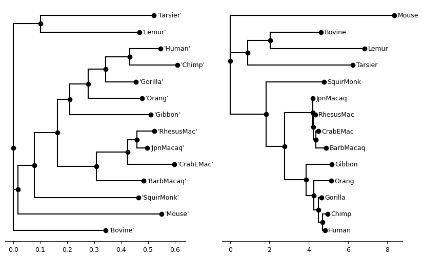

Manipulating trees with phylo2vec¶

Before looking at how to use the produced trees with phylo2vec, we will quickly visit its main functions.

To import phylo2vec, simply run import phylo2vec

import phylo2vec as p2v

Sampling a random tree¶

The definition of phylo2vec makes it very convenient to rapidly sample large, or lots of, trees.

Use sample_vector to sample a random tree topology.

p2v.sample_vector?

Signature: p2v.sample_vector(n_leaves: int, ordered: bool = False) -> numpy.ndarray
Docstring:
Sample a random tree via Phylo2Vec, in vector form.

Parameters
----------
n_leaves : int
    Number of leaves (>= 2)
ordered : bool, optional
    If True, sample an ordered tree, by default False

    True:
    v_i in {0, 1, ..., i} for i in (0, n_leaves-1)

    False:
    v_i in {0, 1, ..., 2*i} for i in (0, n_leaves-1)

Returns
-------
numpy.ndarray
    Phylo2Vec vector
File:      ~/src/phylo2vec/workshop/.pixi/envs/default/lib/python3.11/site-packages/phylo2vec/utils/vector.py
Type:      function

v5 = p2v.sample_vector(5)
v5

array([0, 1, 4, 4])

Use sample_matrix to sample a random tree (topology + branch lengths)

p2v.sample_matrix?

Signature: p2v.sample_matrix(n_leaves: int, ordered: bool = False) -> numpy.ndarray
Docstring:
Sample a random tree with branch lengths via Phylo2Vec, in matrix form.

Parameters
----------
n_leaves : int
    Number of leaves (>= 2)
ordered : bool, optional
    If True, sample an ordered tree, by default False

Returns
-------
numpy.ndarray
    Phylo2Vec matrix
    Dimensions (n_leaves, 3)
    1st column: Phylo2Vec vector
    2nd and 3rd columns: branch lengths of cherry [i] in the ancestry matrix
File:      ~/src/phylo2vec/workshop/.pixi/envs/default/lib/python3.11/site-packages/phylo2vec/utils/matrix.py
Type:      function

m6 = p2v.sample_matrix(6).round(3)
m6

array([[0.   , 0.007, 0.785],
       [0.   , 0.52 , 0.221],
       [4.   , 0.012, 0.75 ],
       [4.   , 0.452, 0.553],
       [5.   , 0.82 , 0.899]])

Conversion: v <--> Newick¶

Use to_newick to convert a vector to a Newick string.

newick5 = p2v.to_newick(v5)
newick6 = p2v.to_newick(m6)

print(f"Newick from v5: {newick5}")
print(f"Newick from m6: {newick6}")

Newick from v5: ((0,((1,2)5,4)6)7,3)8;
Newick from m6: (((((0:0.007,2:0.785)6:0.52,5:0.221)7:0.012,4:0.75)8:0.452,1:0.553)9:0.82,3:0.899)10;

Use from_newick to convert a Newick string to a vector.

v5_new = p2v.from_newick(newick5)
print(f"Is v5 equal to v5_new? {np.array_equal(v5, v5_new)}")

m6_new = p2v.from_newick(newick6)
print(f"Is m6 equal to m6_new? {np.array_equal(m6, m6_new)}")

Is v5 equal to v5_new? True
Is m6 equal to m6_new? True

Conversion: v <--> Edge list¶

An intuitive way to represent a tree topology (or any graph) is a list of edges

p2v.to_edges?

Signature: p2v.to_edges(v: numpy.ndarray) -> List[Tuple[int, int]]
Docstring:
Convert a Phylo2Vec vector to an edge list

Each edge is represented as a list of two nodes (child, parent)

Parameters
----------
v : numpy.ndarray
    Phylo2Vec vector

Returns
-------
edges : List[Tuple[int, int]]
    List of (child, parent) edges
File:      ~/src/phylo2vec/workshop/.pixi/envs/default/lib/python3.11/site-packages/phylo2vec/base/edges.py
Type:      function

Use to_edges to convert a vector to a list of tree edges (node1, node2) Use from_edges to convert a list of edges back to a vector

edges5 = p2v.to_edges(v5)
print(edges5)
v5_edges = p2v.from_edges(edges5)
print(f"Is v5 equal to v5_edges? {np.array_equal(v5, v5_edges)}")

[(1, 5), (2, 5), (5, 6), (4, 6), (0, 7), (6, 7), (7, 8), (3, 8)]
Is v5 equal to v5_edges? True

Conversion: v <--> Ancestry matrix¶

An intermediate way between the compact phylo2vec format and the Newick string of representing tree topology is what we call the “ancestry” matrix, a matrix of triplets [child1, child2, parent].

Use to_ancestry to convert a vector to an ancestry matrix

anc5 = p2v.to_ancestry(v5)
anc6 = p2v.to_ancestry(m6[:, 0].astype(int))

print(f"Ancestry from v5:\n{anc5}")
print(f"Ancestry from m6:\n{anc6}")

Ancestry from v5:
[[1 2 5]
 [5 4 6]
 [0 6 7]
 [7 3 8]]
Ancestry from m6:
[[ 0  2  6]
 [ 6  5  7]
 [ 7  4  8]
 [ 8  1  9]
 [ 9  3 10]]

The ancestry matrix is also useful to understand the order of the branch lengths in the matrix format. For a row $i$ of m6, the branch lengths are those of the children of triplet $i$ .

plot_tree(Tree(newick6))

<Axes: >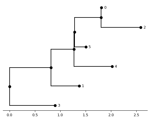

Back to our primate trees¶

phylo2vec works on rooted integer trees, while both rapidNJ and IQ-TREE produce unrooted trees. Before loading the produced trees into phylo2vec, we need to:

Root the trees (we will here use Mouse, as we assume that it is the most distantly related taxon). For that, we use the set_outgroup function of ete3
Apply a mapping of string to integer to keep the same information while having an integer tree. For that, we use the create_label_mapping function of phylo2vec

from phylo2vec.utils.newick import create_label_mapping


def load_tree(file, root=None, with_branch_lengths=True):
    # Load into ete3 for potential re-rooting
    tr = Tree(file)
    # Reroot
    if root:
        tr.set_outgroup(root)
    # Write the tree back to Newick
    if with_branch_lengths:
        newick_str = tr.write(format=1, dist_formatter="%.06f")
    else:
        newick_str = tr.write(format=9)

    # Apply a mapping
    newick_int, label_mapping = create_label_mapping(newick_str.replace("'", ""))

    data = {
        "newick_str": newick_str,
        "newick_int": newick_int,
        "label_mapping": dict(sorted(label_mapping.items())),
    }

    # Convert to phylo2vec object
    p2v_obj = p2v.from_newick(newick_int)

    if p2v_obj.ndim == 1:
        # ndim == 1 means it's a vector
        data["v"] = p2v_obj
    elif p2v_obj.ndim == 2:
        # ndim == 2 means it's a matrix
        data["m"] = p2v_obj
        data["v"] = p2v_obj[:, 0].astype(int)
    else:
        raise ValueError("Unexpected ndim in phylo2vec object")
    return data

primate_iqtree_data = load_tree(
    primate_iqtree_file, root="Mouse", with_branch_lengths=False
)

primate_iqtree_data

{'newick_str': '(Mouse,(((Bovine,Lemur),Tarsier),(SquirMonk,((JpnMacaq,(RhesusMac,(CrabEMac,BarbMacaq))),(Gibbon,(Orang,(Gorilla,(Chimp,Human))))))));',
 'newick_int': '(0,(((1,2),3),(4,((5,(6,(7,8))),(9,(10,(11,(12,13))))))));',
 'label_mapping': {0: 'Mouse',
  1: 'Bovine',
  2: 'Lemur',
  3: 'Tarsier',
  4: 'SquirMonk',
  5: 'JpnMacaq',
  6: 'RhesusMac',
  7: 'CrabEMac',
  8: 'BarbMacaq',
  9: 'Gibbon',
  10: 'Orang',
  11: 'Gorilla',
  12: 'Chimp',
  13: 'Human'},
 'v': array([ 0,  1,  3,  5,  4,  5,  6,  7, 11,  9, 10, 11, 12])}

Here:

newick_str is the orginal tree (without branch lengths)
newick_int is the same tree, but with using integers to represent leaves
label_mapping is a dict of the integer-to-taxon mapping
v is the phylo2vec vector extracted from newick_int

plot_tree(Tree(primate_iqtree_data["newick_int"]))

<Axes: >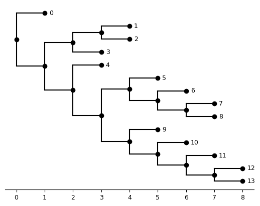

One of the core functions of phylo2vec is to convert several objects representing trees to this compact vector format, and vice versa.

import phylo2vec as p2v

v = primate_iqtree_data["v"]
print(f"Vector representation: {repr(v)}")
print(f"Original integer Newick: {primate_iqtree_data['newick_int']}")
print(f"Converted integer Newick: {p2v.to_newick(v)}")

Vector representation: array([ 0,  1,  3,  5,  4,  5,  6,  7, 11,  9, 10, 11, 12])
Original integer Newick: (0,(((1,2),3),(4,((5,(6,(7,8))),(9,(10,(11,(12,13))))))));
Converted integer Newick: (0,(((1,2)23,3)24,(4,((5,(6,(7,8)18)19)20,(9,(10,(11,(12,13)14)15)16)17)21)22)25)26;

Another example is a list of graph edges of the form (child, parent)

edges = p2v.to_edges(v)
print(f"Edge list: {edges}")
new_v = p2v.from_edges(edges)
assert np.array_equal(v, new_v)

Edge list: [(12, 14), (13, 14), (11, 15), (14, 15), (10, 16), (15, 16), (9, 17), (16, 17), (7, 18), (8, 18), (6, 19), (18, 19), (5, 20), (19, 20), (20, 21), (17, 21), (4, 22), (21, 22), (1, 23), (2, 23), (23, 24), (3, 24), (24, 25), (22, 25), (0, 26), (25, 26)]

primate_rapidnj_data = load_tree(primate_rapidnj_file, root="'Mouse'")

primate_rapidnj_data

{'newick_str': "('Mouse':0.267050,((((((('Human':0.115680,'Chimp':0.178270):0.088192,'Gorilla':0.112280):0.066043,'Orang':0.201080):0.068184,'Gibbon':0.301130):0.045591,((('RhesusMac':0.066186,'JpnMacaq':0.038473):0.032833,'CrabEMac':0.172450):0.116060,'BarbMacaq':0.174200):0.145580):0.085270,'SquirMonk':0.386660):0.061420,(('Tarsier':0.420990,'Lemur':0.367210):0.101000,'Bovine':0.343560):0.017041):0.267050);",
 'newick_int': '(0:0.267050,(((((((1:0.115680,2:0.178270):0.088192,3:0.112280):0.066043,4:0.201080):0.068184,5:0.301130):0.045591,(((6:0.066186,7:0.038473):0.032833,8:0.172450):0.116060,9:0.174200):0.145580):0.085270,10:0.386660):0.061420,((11:0.420990,12:0.367210):0.101000,13:0.343560):0.017041):0.267050);',
 'label_mapping': {0: 'Mouse',
  1: 'Human',
  2: 'Chimp',
  3: 'Gorilla',
  4: 'Orang',
  5: 'Gibbon',
  6: 'RhesusMac',
  7: 'JpnMacaq',
  8: 'CrabEMac',
  9: 'BarbMacaq',
  10: 'SquirMonk',
  11: 'Tarsier',
  12: 'Lemur',
  13: 'Bovine'},
 'm': array([[0.0000e+00, 4.2099e-01, 3.6721e-01],
        [1.0000e+00, 1.0100e-01, 3.4356e-01],
        [3.0000e+00, 6.6186e-02, 3.8473e-02],
        [5.0000e+00, 3.2833e-02, 1.7245e-01],
        [7.0000e+00, 1.1606e-01, 1.7420e-01],
        [9.0000e+00, 1.1568e-01, 1.7827e-01],
        [6.0000e+00, 8.8192e-02, 1.1228e-01],
        [8.0000e+00, 6.6043e-02, 2.0108e-01],
        [1.0000e+01, 6.8184e-02, 3.0113e-01],
        [1.7000e+01, 4.5591e-02, 1.4558e-01],
        [1.9000e+01, 8.5270e-02, 3.8666e-01],
        [1.1000e+01, 6.1420e-02, 1.7041e-02],
        [1.3000e+01, 2.6705e-01, 2.6705e-01]]),
 'v': array([ 0,  1,  3,  5,  7,  9,  6,  8, 10, 17, 19, 11, 13])}

Advantages of phylo2vec package¶

Sampling speed¶

Example of a simple benchmark against ete3 and IQ-TREE.

We use timeit for a simple benchmark of python commands.

We use time inside of pixi to minimise overhead when calling iqtree. We use the quiet option to limit print messages. Note that this benchmark is an upper bound of the actual time due to I/O operations.

big_n = 10000
# Sample a topology
%timeit p2v.sample_vector(big_n)
%timeit tr = Tree(); tr.populate(big_n)
# Sample a topology with branch lengths
%timeit p2v.sample_matrix(big_n)
!pixi run -- time iqtree -ru 10000 10000.tree -redo --quiet

485 μs ± 3.63 μs per loop (mean ± std. dev. of 7 runs, 1,000 loops each)
25.7 ms ± 444 μs per loop (mean ± std. dev. of 7 runs, 10 loops each)
524 μs ± 613 ns per loop (mean ± std. dev. of 7 runs, 1,000 loops each)
⠁ activating environment                                                        0.01user 0.01system 0:00.03elapsed 96%CPU (0avgtext+0avgdata 16404maxresident)k
0inputs+672outputs (0major+2458minor)pagefaults 0swaps

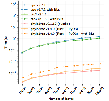
Sampling speed of phylo2vec and other libraries. Author: Neil Scheidwasser. Source: Pandemic preparedness in a vector, PhD thesis (in preparation, 2025). License: CC BY 4.0.

Memory efficiency¶

Example of a memory benchmark against the Newick-formatted outputs from IQ-TREE and rapidNJ.

We use sys.getsizeof to evaluate the size of standard python objects, and the nbytes attribute to evaluate the size of NumPy array (the base for phylo2vec objects in Python).

import sys

print(
    f"Newick with branch lengths:\nNewick = {sys.getsizeof(primate_rapidnj_data['newick_str'])}, P2V = {primate_rapidnj_data['m'].nbytes}"
)
print(
    f"Newick without branch lengths:\nNewick = {sys.getsizeof(primate_iqtree_data['newick_str'])}, P2V = {primate_iqtree_data['v'].nbytes}"
)

Newick with branch lengths:
Newick = 445, P2V = 312
Newick without branch lengths:
Newick = 183, P2V = 104

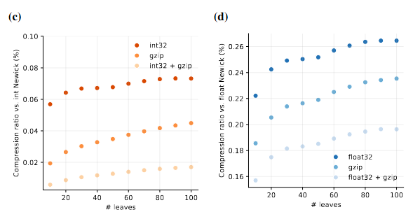
File size ratio 10,000 random tree topologies (resp. trees with branch lengths) with coronavirus taxa saved:

as a plain-text file (reference)
a hierarchical data format (HDF) file containing the trees as an array of phylo2vec vectors (resp. matrices) + and a mapping of taxon-to-integer labels

Figure source: Pandemic preparedness in a vector, PhD thesis (in preparation, 2025). Author: Neil Scheidwasser. License: CC BY 4.0.

Phylo2Vec Workshop

Exercises